Hands-On Lattice and Longitudinal Calculations

During the CAS 2021 in Chavannes de Bogis (Switzerland), we will use Python as scripting language for the Hands-On Lattice and Longitudinal Calculations. We kindly ask you to make some homework before coming to to prepare yourself (and your laptop) for the course.

We strongly suggest to use Python for the course.

A basic knowledge of Python is assumed, therefore if you are not familiar with it you can find, in the following sections, few resources to fill the gap.

During the course we will use Python3 in a Jupyter notebook and, mostly, the numpy and matplotlib packages. We will explain in the following sections how to install this software on your laptops.

After a short introduction where we provided some useful links to get familiar with Python, we will focus on the software setup.

To get a better idea of the level of the Python knowledge needed for the course you can browse the Primer of the Hands-on exercises. Do not worry about the theory for the moment (it will be discussed in details during the school) but focus on the Python syntax and data types (tuples, lists,…).

A (very) short introduction to Python

You can find several nice courses, videos and resources on the internet. Here you are a couple of suggestions

Test Python on a web page

If you are not familiar with Python and you have not it installed on your laptop, you can start playing with simple python snippets on the web: without installing any special software you can connect, e.g., to

jupyterLab

and test the following commands

import numpy as np
# Matrix definition
Omega=np.array([[0, 1],[-1,0]])
M=np.array([[1, 0],[1,1]])

# Sum and multiplication of matrices
Omega - M.T @ Omega @ M
# M.T means the "traspose of M".

# Function definition
def Q(f=1):
    return np.array([[1, 0],[-1/f,1]])

#Eigenvalues and eigenvectors
np.linalg.eig(M)

You can compare and check your output with the ones here.

Python packages

You can leverage python’s capability by exploring a galaxy of packages. Below you can find the most useful for our course (focus mostly on numpy and matplotlib) and some very popular ones.

The numpy package

To get familiar with the numpy package have a look at the following summary poster.

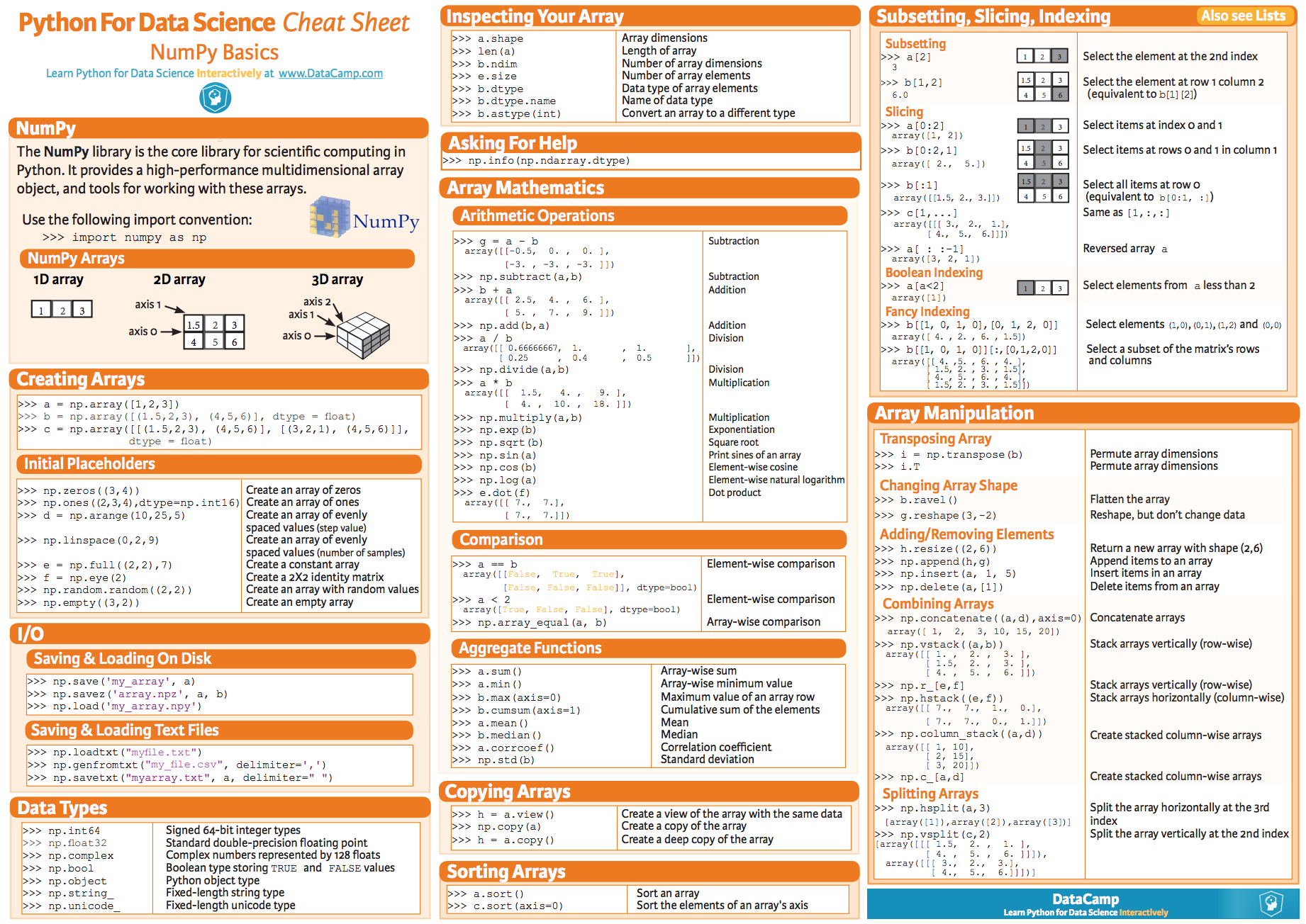
You can google many other resources, but the one presented of the poster covers the set of instructions you should familiar with.

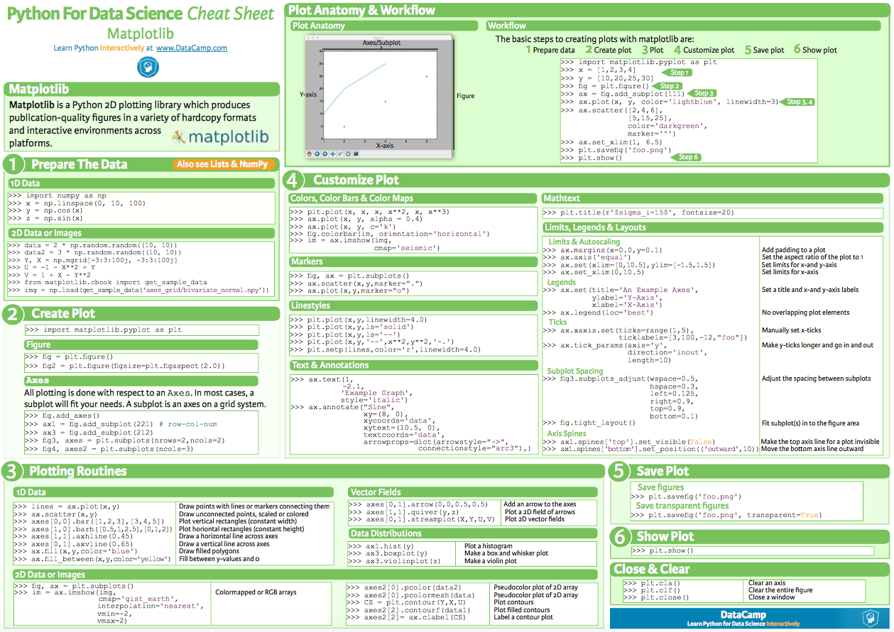
The matplotlib package

To get familiar with the matplotlib package have a look at the following summary poster.

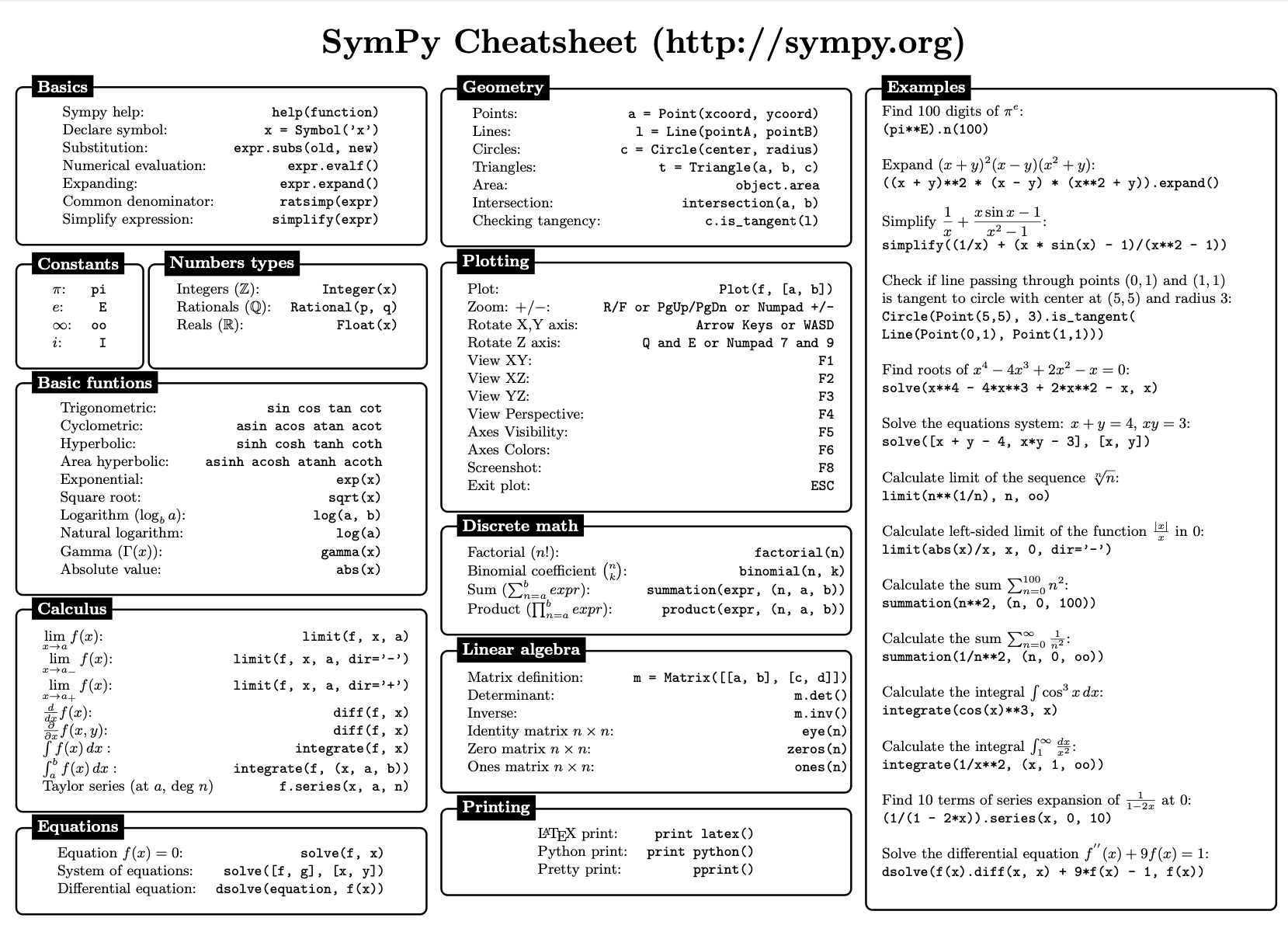
The sympy package

To get familiar with the sympy package have a look at the following summary poster.

The linalg module

To get familiar with the Linear Algebra (linalg) module have a look at the following summary poster.

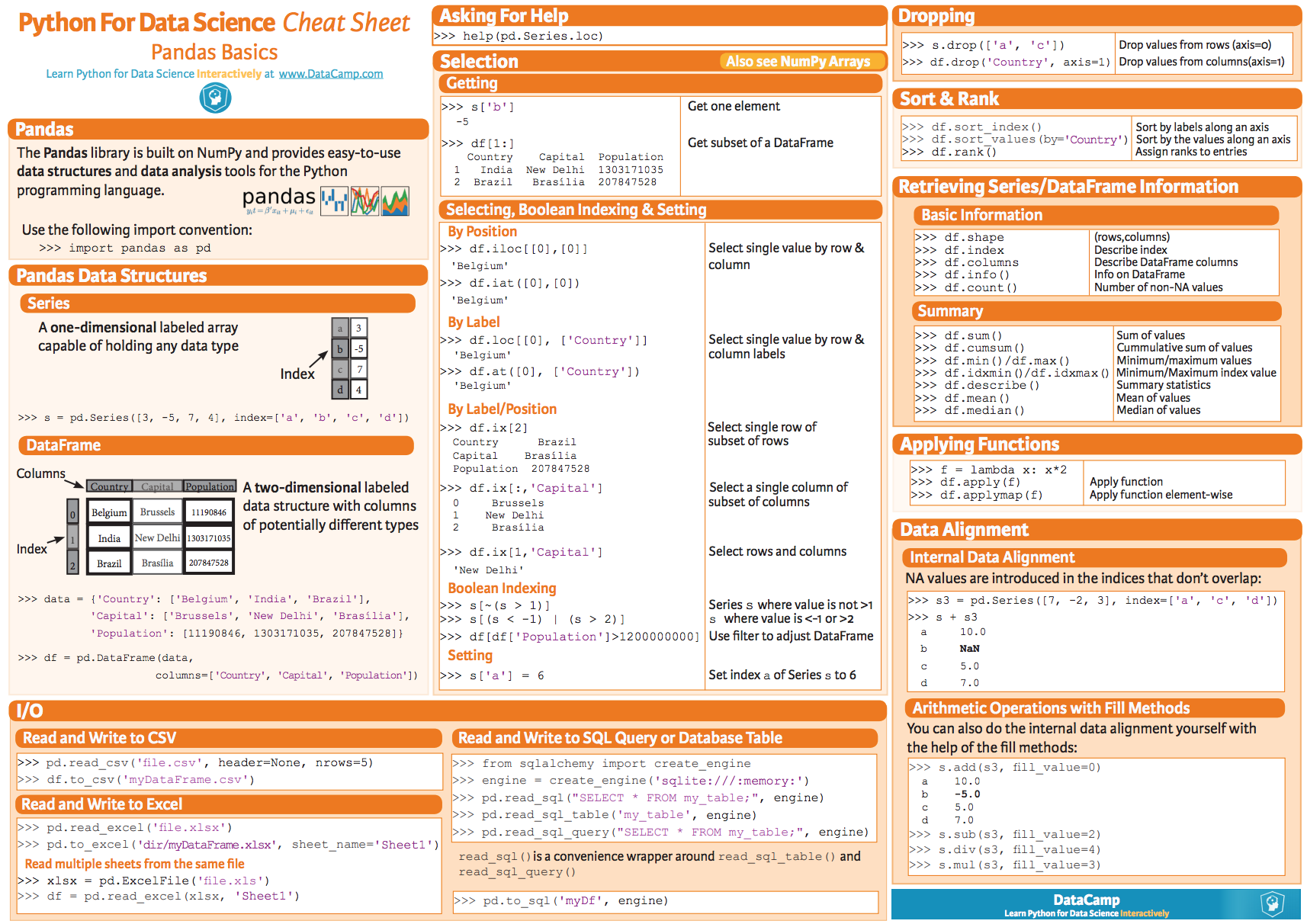
The pandas package (optional)

To get familiar with the pandas package have a look at the following summary poster.

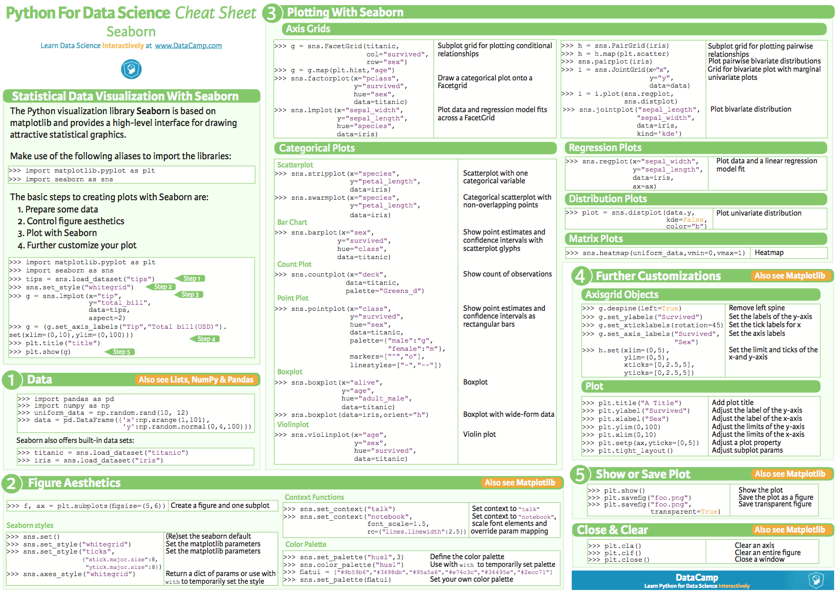
The seaborn package (optional)

To get familiar with the seaborn package have a look at the following summary poster.

JupyterLab installation

JupyterLab is a user-friendly environment to work with Python.

You can find an overview on JupyterLab here.

In the following section we will explain how to install a Python on your laptop.

Installation

Please install the Anaconda distribution from
https://www.anaconda.com/distribution/

Please test the following code to check that all packages are correctly installed. Launch Jupyter Lab from a terminal

jupyter lab

You should end-up on your default browser with a page similar to the following:

If you are not familiar with Python, you can start playing with simple python snippets.

Indexing

Generate a random array and select specific elements:

import numpy as np

# Create an array
array1d = np.random.uniform(size=10)
# Print selected elements
print("Entire array: " + str(array1d) + "\n")
print("Specific element: " + str(array1d[5]) + "\n")
print("Last element: " + str(array1d[-1]) + "\n")
print("Specific elements: " + str(array1d[3:7]) + "\n")
print("First 5 elements array: " + str(array1d[:5]) + "\n")
print("Last 5 elements array: " + str(array1d[5:]) + "\n")

will result in, e.g.:

Entire array: [0.09402447 0.05647033 0.79670378 0.60573004 0.81588777 0.97863634 0.51376609 0.19763518 0.7649532  0.59285346]

Specific element: 0.9786363385079204

Last element: 0.5928534616865488

Specific elements: [0.60573004 0.81588777 0.97863634 0.51376609]

First 5 elements array: [0.09402447 0.05647033 0.79670378 0.60573004 0.81588777]

Last 5 elements array: [0.97863634 0.51376609 0.19763518 0.7649532  0.59285346]

Implicit loops

In contrast to programming languages like C++, Python can handle vectors. No loop is required, e.g. to multiply each element with a constant or squaring it:

import numpy as np

# Create an array
array1d = np.random.uniform(size=10)

print("Entire array: " + str(array1d) + "\n")
print("Each element muliplied by 5: " + str(5 * array1d) + "\n")
print("Each element squared: " + str(array1d**2) + "\n")
print("Square root of each element: " + str(np.sqrt(array1d)) + "\n")

will result in, e.g.:

Entire array: [0.2240143  0.35153156 0.68864907 0.14062298 0.77280195 0.26872206 0.9135403  0.8776261 0.26158576 0.93883652]

Each element muliplied by 5: [1.12007151 1.75765782 3.44324537 0.70311488 3.86400975 1.34361029 4.56770149 4.3881305 1.30792879 4.69418259]

Each element squared: [0.05018241 0.12357444 0.47423755 0.01977482 0.59722285 0.07221154 0.83455588 0.77022757 0.06842711 0.88141401]

Square root of each element: [0.47330149 0.59290097 0.82984883 0.3749973  0.87909155 0.51838408 0.95579302 0.936817 0.51145455 0.96893577]

Or you can perform some linear algebra tests:

import numpy as np
import pandas as pd
from matplotlib import pyplot as plt
import seaborn as sns
import sympy as sy

# Matrix definition
Omega=np.array([[0, 1],[-1,0]])
M=np.array([[1, 0],[1,1]])

# Sum and multiplication of matrices
Omega - M.T @ Omega @ M
# M.T means the "traspose of M".

# Function definition
def Q(f=1):
    return np.array([[1, 0],[-1/f,1]])

#Eigenvalues and eigenvectors
np.linalg.eig(M)

Plotting

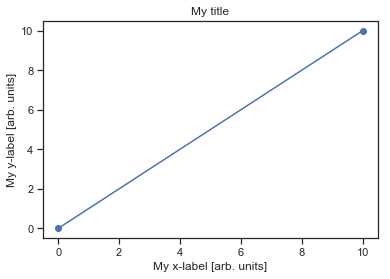
Or you can test a simple plot:

# check a simple plot
%matplotlib inline

plt.plot([0,10],[0,10],'ob-')
plt.xlabel('My x-label [arb. units]')
plt.ylabel('My y-label [arb. units]')
plt.title('My title')

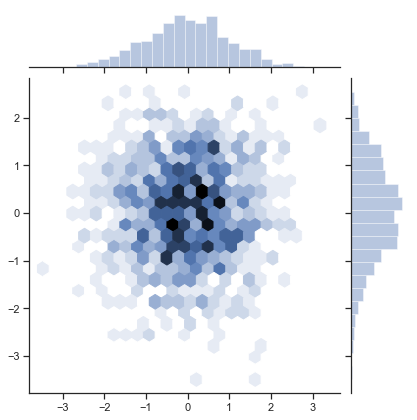
Or something fancier:

# an sns plot
sns.set(style="ticks")
rs = np.random.RandomState(11)
x = rs.normal(size=1000)
y = rs.normal(size=1000)
sns.jointplot(x=x, y=y, kind="hex")

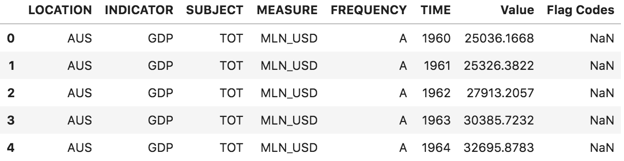
Or you can import from the internet some information in a pandas dataframe:

# a simple pandas dataframe (GDP world statistics)
myDF=pd.read_csv('https://stats.oecd.org/sdmx-json/data/DP_LIVE/.GDP.../OECD?contentType=csv&detail=code&separator=comma&csv-lang=en')
myDF[(myDF['TIME']==2018) & (myDF['MEASURE']=='MLN_USD')]
myDF.head()

that gives

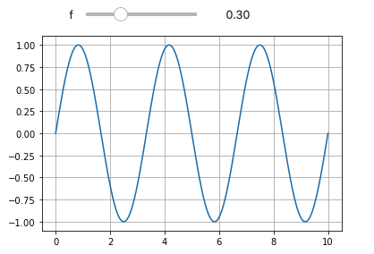
Animations

Please check that the following code is running or your machine.

# to have the animation you need to configure properly
# your jupyter lab
# From 
# https://towardsdatascience.com/interactive-controls-for-jupyter-notebooks-f5c94829aee6

# > pip install ipywidgets
# > jupyter nbextension enable --py widgetsnbextension
# > jupyter labextension install @jupyter-widgets/jupyterlab-manager

# Possibly you need also nodejs 
# https://anaconda.org/conda-forge/nodejs
# > conda install -c conda-forge nodejs 


import numpy as np
import matplotlib.pyplot as plt
from ipywidgets import interactive

t = np.linspace(0,10,1000)
def plotIt(f):
    plt.plot(t, np.sin(2*np.pi*f*t))
    plt.grid(True)
    
interactive_plot = interactive(plotIt,f=(0,1,.1),continuous_update=True)
output = interactive_plot.children[-1]
output.layout.height = '300px'
interactive_plot