RF CAS 2023 - Longitudinal Tracking Hands-On Exercises

TL;DR

0. You’ll need your own laptop, contact the RF CAS if you don’t have one.
1. Install a Python3 distribution, we recommend Anaconda or Python>=3.8.
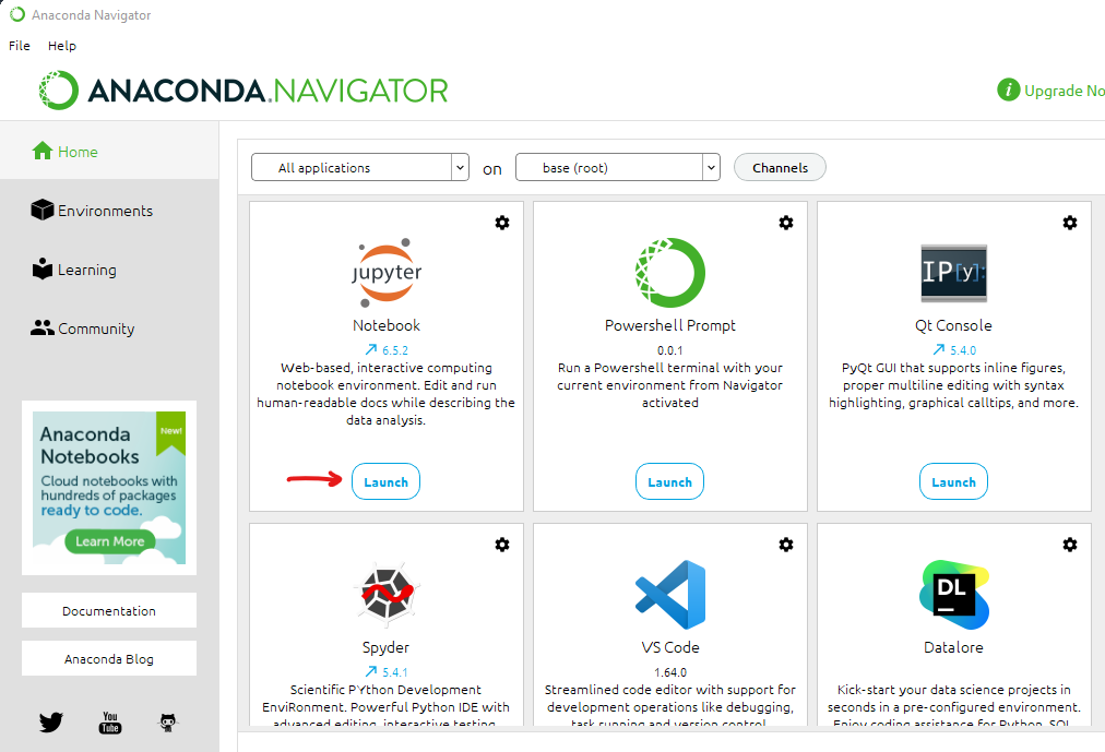
2. Open the Anaconda Navigator and run Jupyter Notebook

3. Create a folder for the RF CAS and make a notebook. Install BLonD by running pip install blond (tip: Shift+Enter to run the cell)

4. You are done! The install command is required only once and doesn’t need to be called for every notebook.
5. To verify the setup, run the blond.test() function after importing.

Introduction

During the RF CAS 2023 in Berlin (Germany), we will use Python as scripting language for the Longitudinal Tracking Hands-on Exercises. We kindly ask you to make some homework before coming to prepare yourself (and your laptop) for the course.

A basic knowledge of Python is assumed, therefore if you are not familiar with it you can find, in the following sections, few resources to fill the gap. During the school, feel free to ask questions to the tutors outside of the hands-on sessions. Should you require some help, we will be pleased to discuss over coffee or in the evening after the courses.

During the course we will use Python3 in a Jupyter notebook for the development. The longitudinal tracking code BLonD will also be used, including the numpy and matplotlib packages as dependencies. We will explain in the following sections how to install this software on your laptops.

After a short introduction where we provided some useful links to get familiar with Python, we will focus on the software setup.

The layout of this document is the following:

1. Installation instructions
2. An introduction to Python
3. More information to go beyond

1. Installation instructions

With Anaconda

0. You’ll need your own laptop, contact the RF CAS if you don’t have one.
1. Install a Python3 distribution, we recommend Anaconda or Python>=3.8.
2. Open the Anaconda Navigator and run Jupyter Notebook

3. Create a folder for the RF CAS and make a notebook. Install BLonD by running pip install blond (tip: Shift+Enter to run the cell)

4. You are done! The install command is required only once and doesn’t need to be called for every notebook.
5. To verify the setup, run the blond.test() function after importing.

With a default python installation

0. Install Python from the official page
1. Open a terminal and go to your favorite folder
2. Create an python environment specific for the tracking hands-on, and activate it

python -m venv env
source env/bin/activate

3. Install BLonD and the jupyter

pip install blond jupyter

4. Run a jupyter notebook instance

jupyter notebook .

If you are willing to know more about BLonD, visit the official repository.

The README also provides instructions on how to install a more efficient compiled version of BLonD.

2. An introduction to Python

Please have a look to the following notebook. Getting experienced with the content of the notebook will make you efficient during the hands-on.

Indexing

Generate a random array and select specific elements:

import numpy as np

# Create an array
array1d = np.random.uniform(size=10)
# Print selected elements
print("Entire array: " + str(array1d) + "\n")
print("Specific element: " + str(array1d[5]) + "\n")
print("Last element: " + str(array1d[-1]) + "\n")
print("Specific elements: " + str(array1d[3:7]) + "\n")
print("First 5 elements array: " + str(array1d[:5]) + "\n")
print("Last 5 elements array: " + str(array1d[5:]) + "\n")

will result in, e.g.:

Entire array: [0.09402447 0.05647033 0.79670378 0.60573004 0.81588777 0.97863634 0.51376609 0.19763518 0.7649532  0.59285346]

Specific element: 0.9786363385079204

Last element: 0.5928534616865488

Specific elements: [0.60573004 0.81588777 0.97863634 0.51376609]

First 5 elements array: [0.09402447 0.05647033 0.79670378 0.60573004 0.81588777]

Last 5 elements array: [0.97863634 0.51376609 0.19763518 0.7649532  0.59285346]

Implicit loops

In contrast to programming languages like C++, Python can handle vectors. No loop is required, e.g. to multiply each element with a constant or squaring it:

import numpy as np

# Create an array
array1d = np.random.uniform(size=10)

print("Entire array: " + str(array1d) + "\n")
print("Each element muliplied by 5: " + str(5 * array1d) + "\n")
print("Each element squared: " + str(array1d**2) + "\n")
print("Square root of each element: " + str(np.sqrt(array1d)) + "\n")

will result in, e.g.:

Entire array: [0.2240143  0.35153156 0.68864907 0.14062298 0.77280195 0.26872206 0.9135403  0.8776261 0.26158576 0.93883652]

Each element muliplied by 5: [1.12007151 1.75765782 3.44324537 0.70311488 3.86400975 1.34361029 4.56770149 4.3881305 1.30792879 4.69418259]

Each element squared: [0.05018241 0.12357444 0.47423755 0.01977482 0.59722285 0.07221154 0.83455588 0.77022757 0.06842711 0.88141401]

Square root of each element: [0.47330149 0.59290097 0.82984883 0.3749973  0.87909155 0.51838408 0.95579302 0.936817 0.51145455 0.96893577]

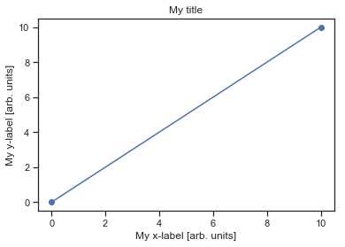
Plotting

Or you can test a simple plot:

import matplotlib.pyplot as plt

# check a simple plot
%matplotlib inline

plt.plot([0,10],[0,10],'ob-')
plt.xlabel('My x-label [arb. units]')
plt.ylabel('My y-label [arb. units]')
plt.title('My title')

3. More information to go beyond

Python packages

You can leverage python’s capability by exploring a galaxy of packages. Below you can find the most useful for our course (focus mostly on numpy, scipy and matplotlib) and some very popular ones.

The numpy package

To get familiar with the numpy package have a look at the following summary poster.

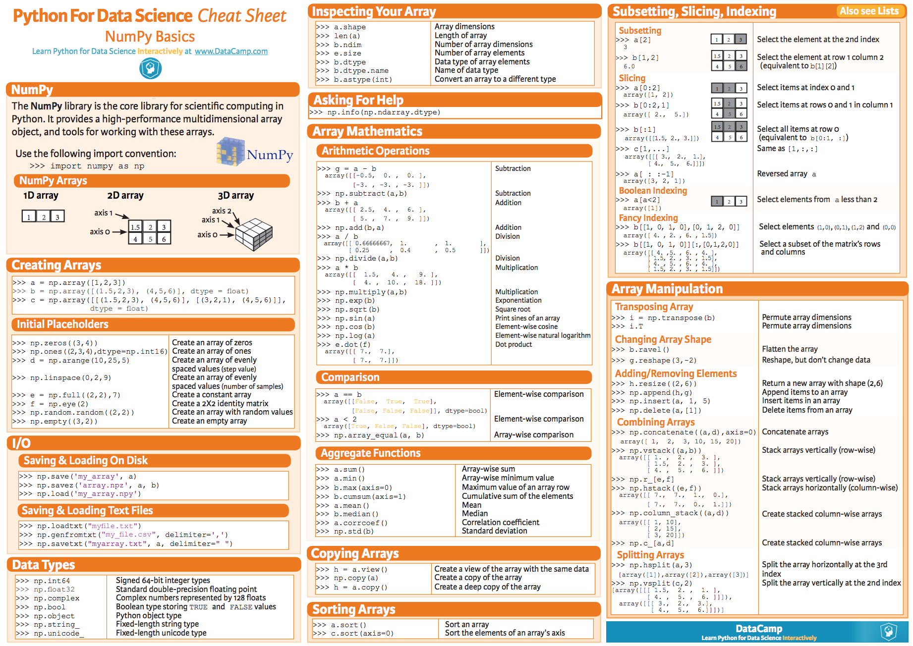
You can google many other resources, but the one presented of the poster covers the set of instructions you should familiar with.

The scipy package

To get familiar with the scipy package have a look at the following summary poster.

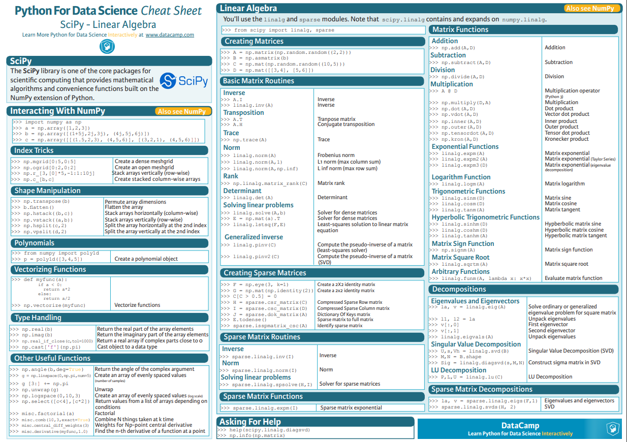
You can google many other resources, but the one presented of the poster covers the set of instructions you should familiar with.

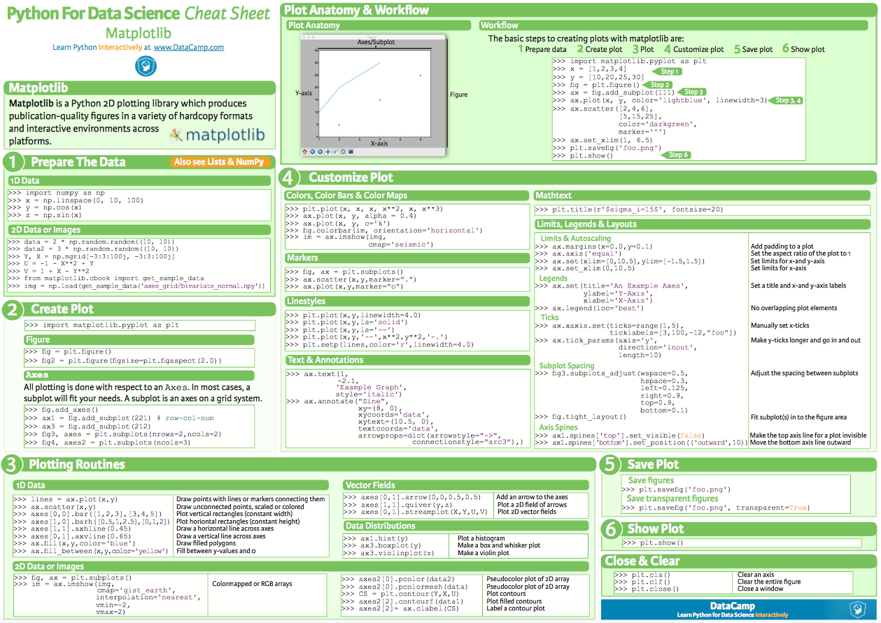
The matplotlib package

To get familiar with the matplotlib package have a look at the following summary poster.

Final words