introduction

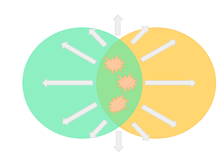
Hot and dense medium created at the LHC
Commonly referred to as the Quark-Gluon Plasma (QGP)
Difference of pressure gradients along different axes drive flow of particles
Gives rise to anisotropic distribution

anisotropic flow

Fourier decomposition of azimuthal distribution of emitted particles [Voloshin, S. et al. Z.Phys. C70 (1996)]
\[ \frac{\mathrm{d}N}{\mathrm{d} \varphi} \propto f(\varphi) = \frac{1}{2 \pi} [1 + 2 \sum^\infty_{n=1} v_n \cos (n[\varphi - \Psi_n])]\]
with
\[ v_n = \langle \cos (n [\varphi - \Psi_n]) \rangle \]

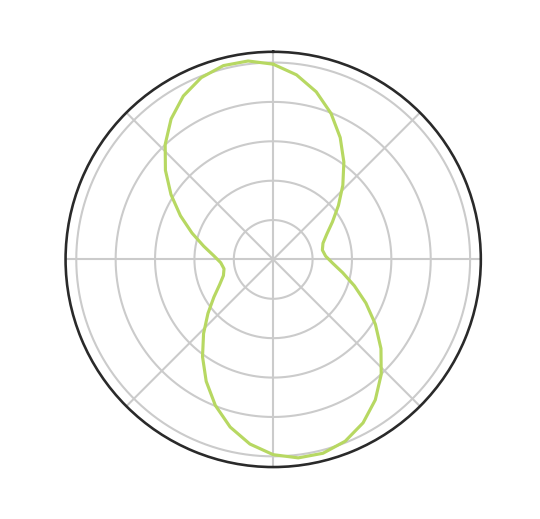
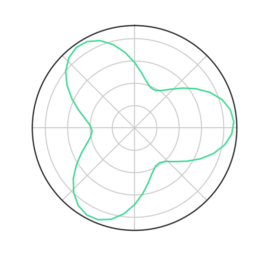
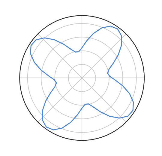
$ v_2 $

$ v_3 $

$ v_1 $

$ v_4 $

anisotropic flow

flow as a function of pseudorapidity

Figure: [ALICE Collaboration, Phys.Lett. B762 (2016)]

$ v_n (\eta) $ give unique information about the hot and dense medium
Forward rapidities
[Phys.Rev.Lett. 116 (2016) no.21, 212301][Phys.Rev. C90 (2014) no.4, 044904]
- Possible change in $ \eta /s $
- Shorter lifetime in the QGP phase
  - Hadronic viscosity play larger role

flow as a function of pseudorapidity

This talk:

Using Generic Framework [Bilandzic, Ante et al., Phys.Rev. C89 (2014)] w. different combinations of sub-events
Run 2 measurements w. more statistics
Significant improvement of systematics

Figure: [ALICE Collaboration, Phys.Lett. B762 (2016)]

$ v_n (\eta) $ give unique information about the hot and dense medium
Forward rapidities
[Phys.Rev.Lett. 116 (2016) no.21, 212301][Phys.Rev. C90 (2014) no.4, 044904]
- Possible change in $ \eta /s $
- Shorter lifetime in the QGP phase
  - Hadronic viscosity play larger role

experiment

alice

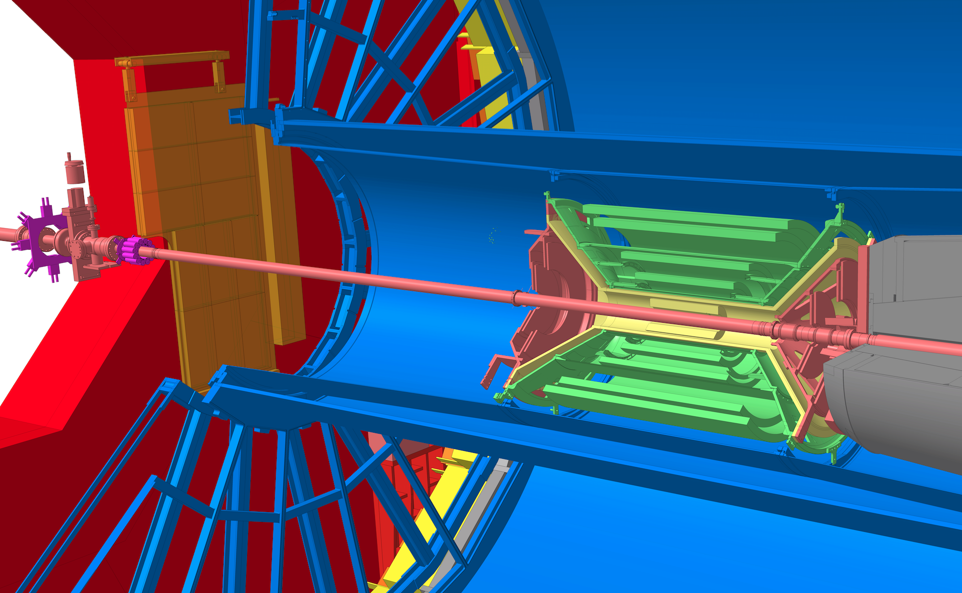
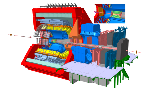
Forward Multiplicity Detector (FMD)

Time Projection Chamber (TPC)

FMD3: $ -3.5 < \eta < -1.7 $
FMD1 & FMD2: $ 1.7 < \eta < 5.0 $
Scintillator

$ -1.1 < \eta < 1.1 $
Tracking

V0 Scintillators

V0A: $ 2.8 < \eta < 5.1 $
V0C: $ -3.7 < \eta < -1.7 $
Trigger

Inner Tracking System (ITS)

Triggering
Tracking

methods

$ v_n $ is calculated using the Generic Framework [Bilandzic, Ante et al., Phys.Rev. C89 (2014)]
Correcting for non-uniform acceptance using weights
- $Q_{n,p} = \sum_j w_j^p e^{in\varphi_j}$
E.g. for 2-particle correlations the equations are
- $ \langle 2 \rangle = \frac{p_{n,1} Q_{-n,1} - q_{0,2}}{p_{0,1} Q_{0,1} - q_{0,2}} $
- $v_n = \sqrt{ \langle \langle 2 \rangle \rangle }$

generic framework

Non-flow: short-range correlations (e.g. jets and resonance decays)
$ \eta $-gaps have shown be useful for removal of non-flow
- using the FMD the gap can increase from $ \Delta \eta \approx 1 $ and up to $ \Delta \eta \approx 4$
E.g. for two particle correlations, the gap case is
$ A \cap B = \emptyset$

non-flow suppression using eta-gaps

How big should a $ \eta $-gap be?

$ \langle 2 \rangle = \frac{p_{n,1}^A Q_{-n,1}^B}{p_{0,1}^A Q_{0,1}^B} $

$ v_n\{2, |\Delta \eta |> x \} = \sqrt{\langle \langle 2 \rangle \rangle } $

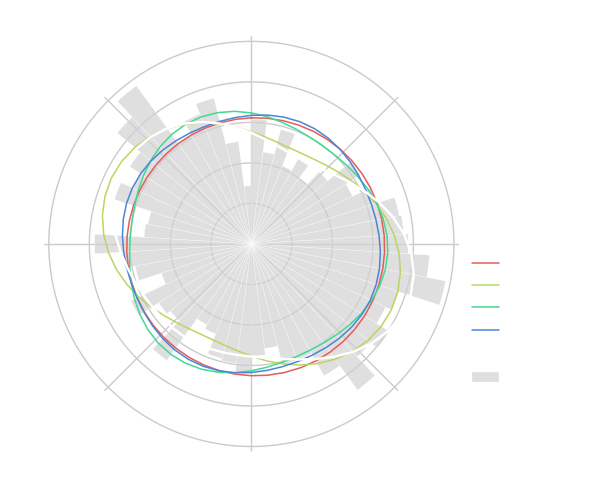
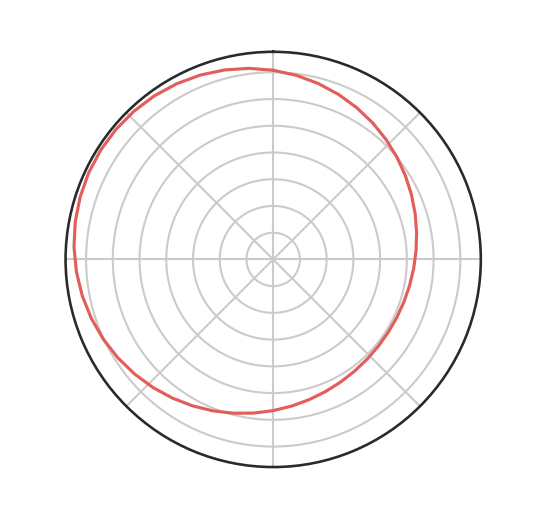
The purely factorizing model express the factorization as,

\[ \langle v_n(\eta_a)v_n(\eta_b) \rangle = \langle v_n(\eta_a)\rangle \langle v_n(\eta_b) \rangle \]

\[ f_2(\Delta \eta) = \langle v_n(\eta_a)\rangle / \langle v_n(\eta_b) \rangle , \Delta \eta = \eta_a - \eta_b\]

For factorization to be true ($f_2(\Delta \eta) = 1$) $ \rightarrow $ need at least a $ \eta $-gap of 2.

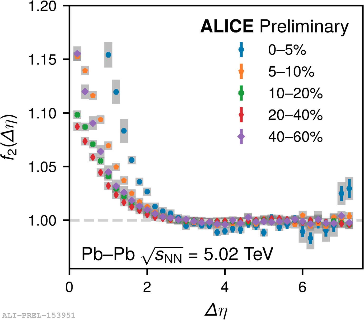
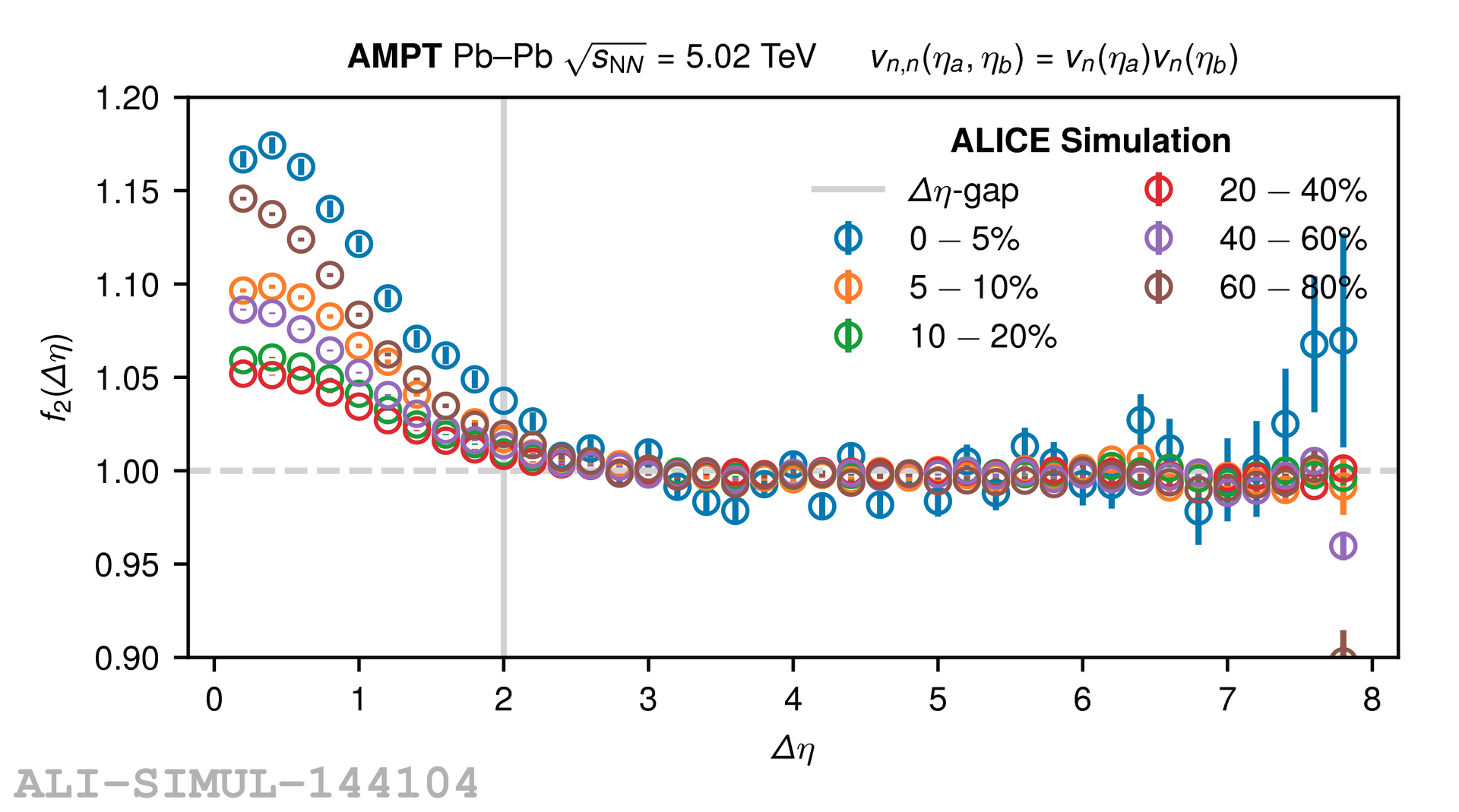
Figure: Factorization from Pb-Pb 5.02 TeV data.

Figure: Factorization from Pb-Pb 5.02 TeV AMPT w. String Melting.

estimating factorising limit

$ \Delta \eta $

Reference particles are chosen from the TPC.
FMD: $ |\Delta \eta| > 2 $
TPC: $|\Delta \eta| > 0$
Example: $ v_n' $ in region B is calculated by, (assuming no decorrelation)

TPC

FMD

v_n^{'B} = \frac{\langle v_n^{'B} v_n^C \rangle }{\sqrt{\langle v_n^B v_n^C \rangle } }

TPC

FMD

Reference particles are chosen from the FMD.
FMD: $ |\Delta \eta| > 4$
TPC: $|\Delta \eta| > 2$
Example: $ v_n' $ in region B is calculated by, (assuming no decorrelation)

v_n^{'B} = \frac{\langle v_n^{'B} v_n^D \rangle }{\sqrt{\langle v_n^A v_n^D \rangle } }

sub-events with pseudorapidity gap

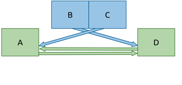
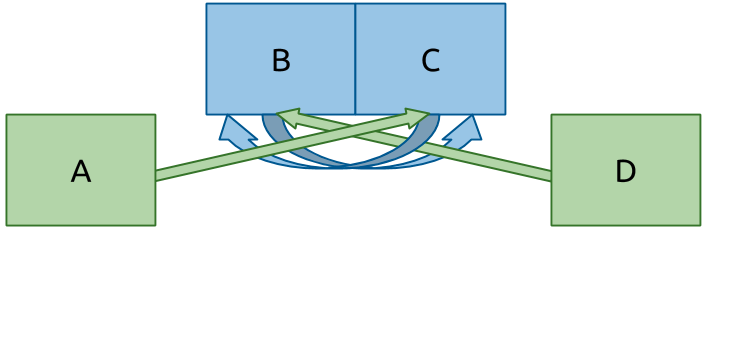
Figures: Beginning of arrow is differential region, end of arrow is reference region

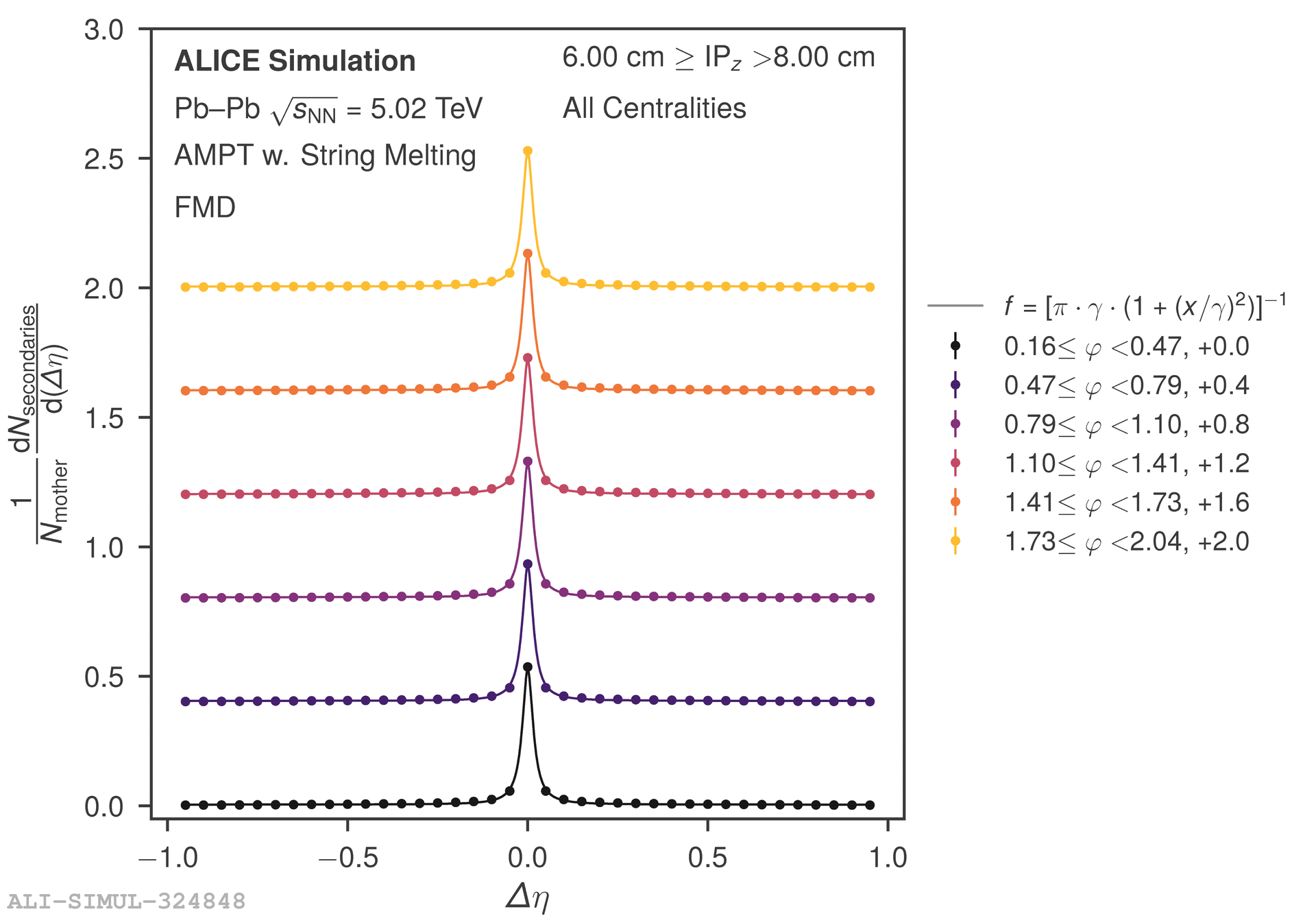
Secondaries in the forward multiplicity detector

Figure: Multiplicity densities of charged particles hitting the SPD and FMD in a HIJING simulation with GEANT3 as transport code for 0 − 5% central events.

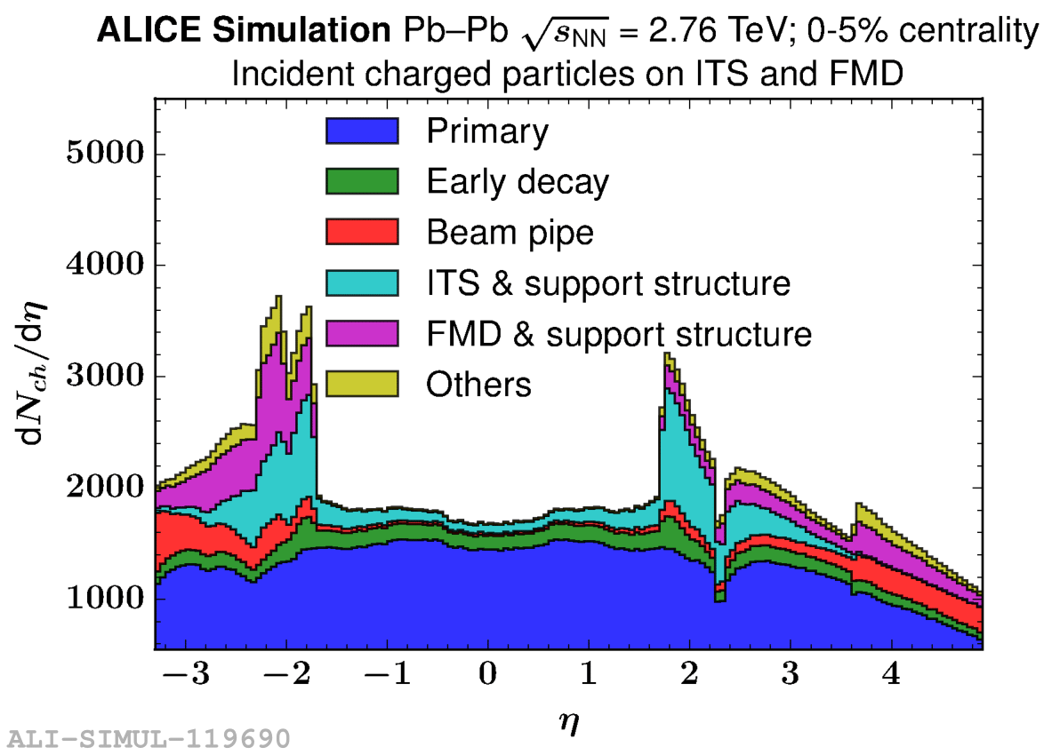
distribution of secondary particles from material

Signal contamination from material interactions (secondaries)
Dilute observation of $ \varphi $
No tracking
- need other method to deconvolve signal

Secondaries distributed around primaries: $$P(\varphi') = f(\varphi) \circ P(\varphi)$$

Observed in the detector: $ \Delta \varphi' = \varphi_1' - \varphi_2$

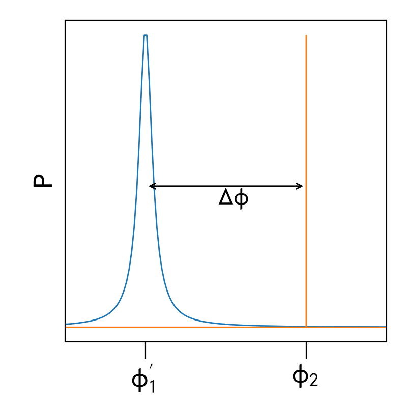
\begin{aligned} \langle \langle v_n' v_n \rangle \rangle^{measured} &= \mathcal{F}(f(\varphi) \circ P(\varphi_1) \circ P(\varphi_2) )\\ &= \mathcal{F}(f(\varphi)) \cdot \mathcal{F}(P(\varphi_1) \circ P(\varphi_2) )\\ &= \mathcal{F} (f(\varphi)) \cdot \langle \langle v_n' v_n \rangle \rangle^{true} \end{aligned}

If we know $\mathcal{F}(f(\varphi)) $ we can extract $ \langle \langle v_n' v_n \rangle \rangle^{true} $

smearing by secondary particles

Figure: Illustration of smearing in $ \varphi $ by secondary particles

$ \Delta \phi $ of observed secondary particle to primary particle

Fourier transform $ f(\varphi) $ for each vertex and $ \eta $ bin

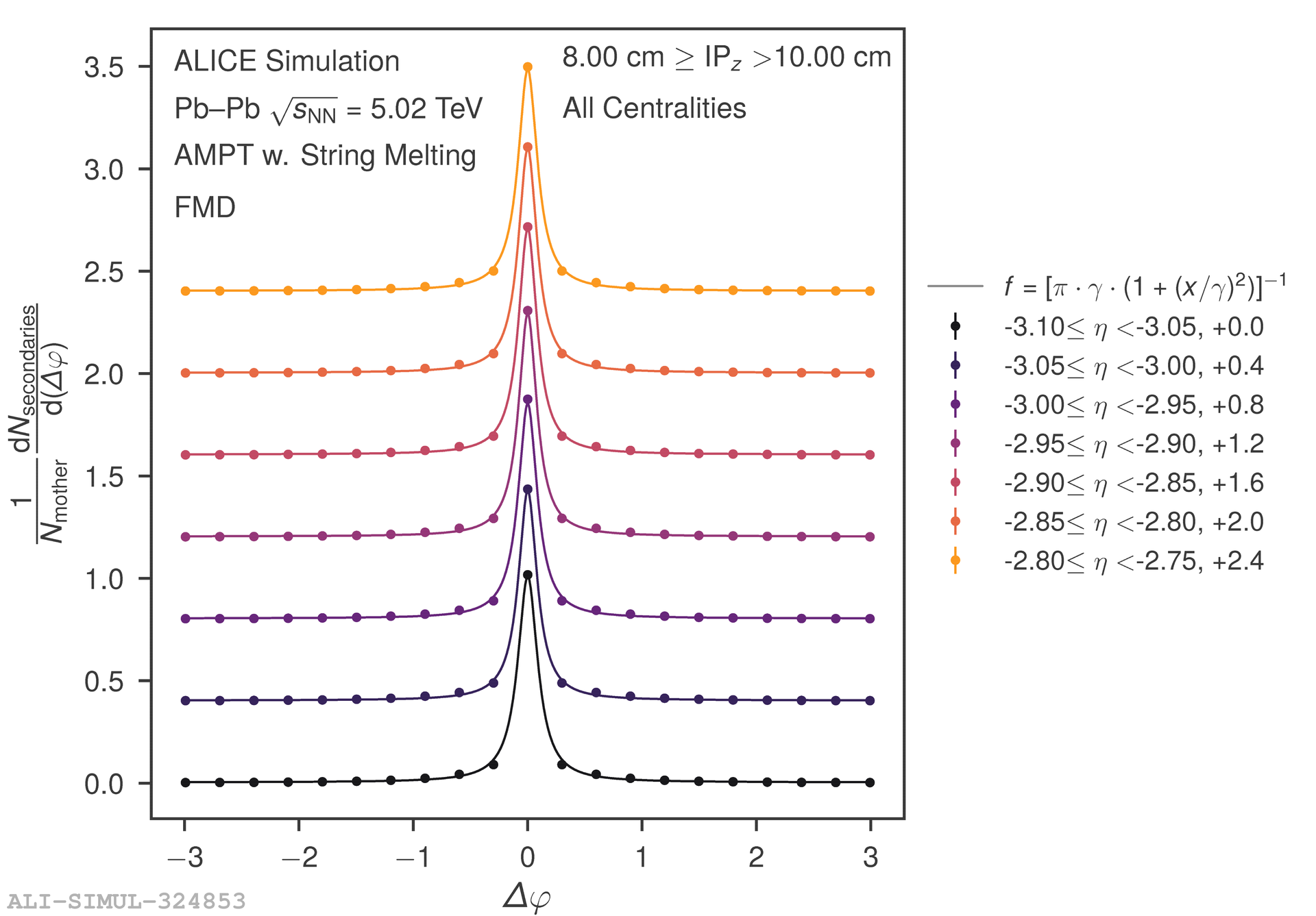
Figure: Distribution of a secondary particle around its primary mother particle. Plots are shifted by a constant.

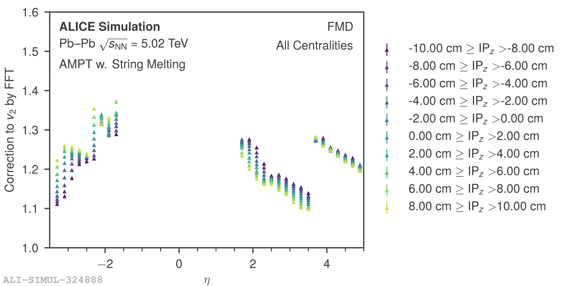
Figure: Correction values to $ v_2 $

distribution of secondaries around primary particles

results

pb-pb

two particle cumulant with small eta-gap

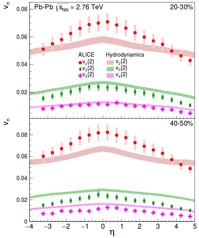
Figure: $ v_n\{2,|\Delta \eta| > 0\}$ as a function of $ \eta $.

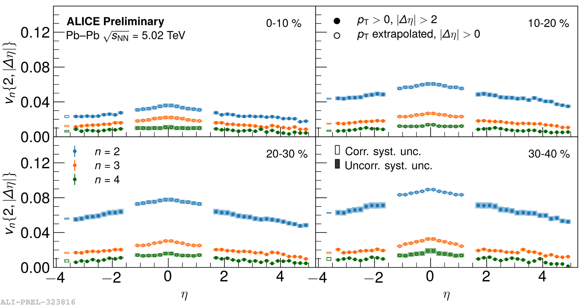
NEW

Ordering of harmonics $ v_2 > v_3 > v_4 $
$ v_n $ increasing from 0 - 40 %
Wide range in $ \eta $ shows $ v_n $ decreasing as a function of $ | \eta | $

two particle cumulant with small eta-gap

Figure: $ v_n\{2,|\Delta \eta| > 0\}$ as a function of $ \eta $.

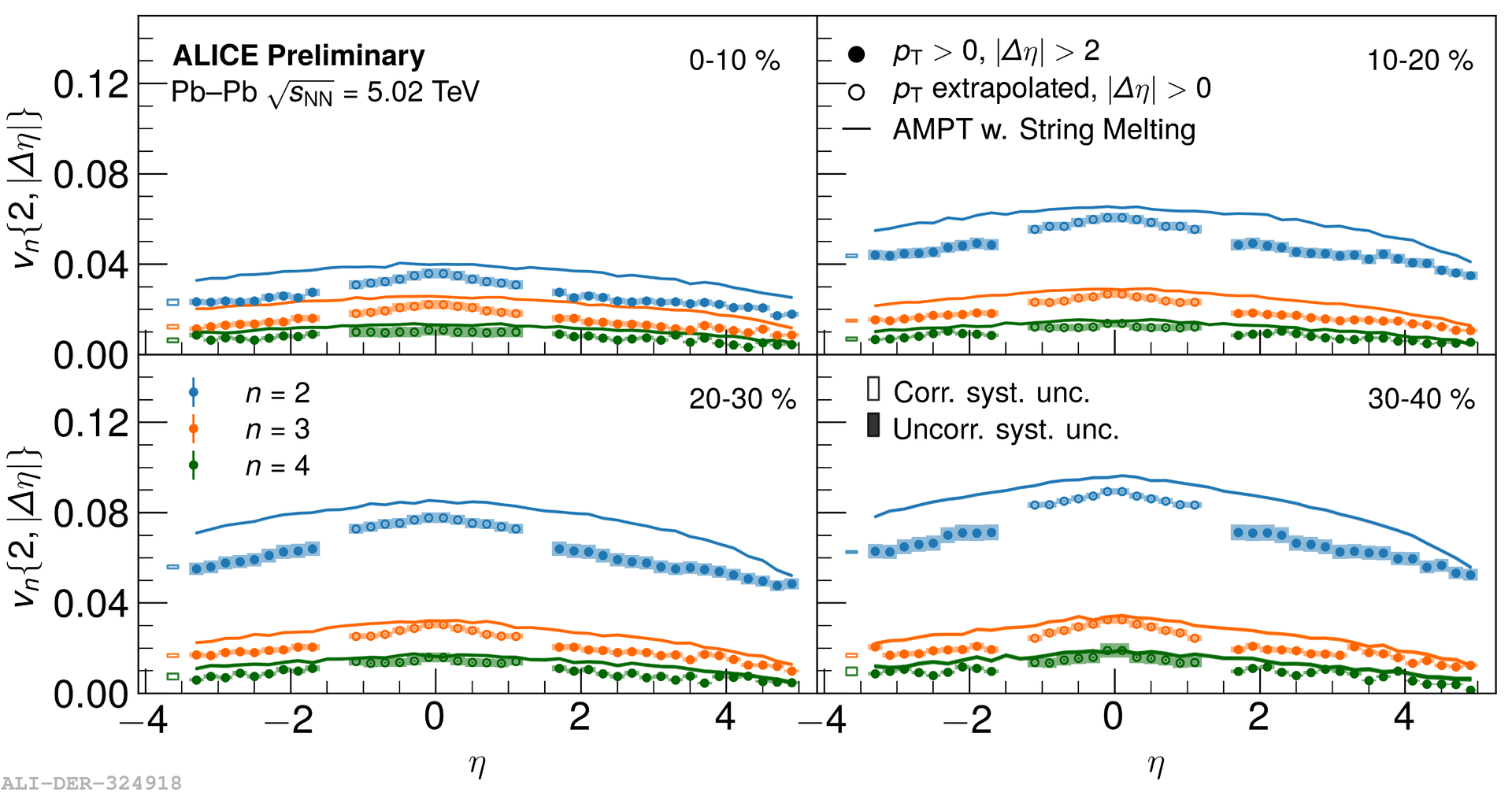
NEW

Ordering of harmonics $ v_2 > v_3 > v_4 $
$ v_n $ increasing from 0 - 40 %
Wide range in $ \eta $ shows $ v_n $ decreasing as a function of $ | \eta | $
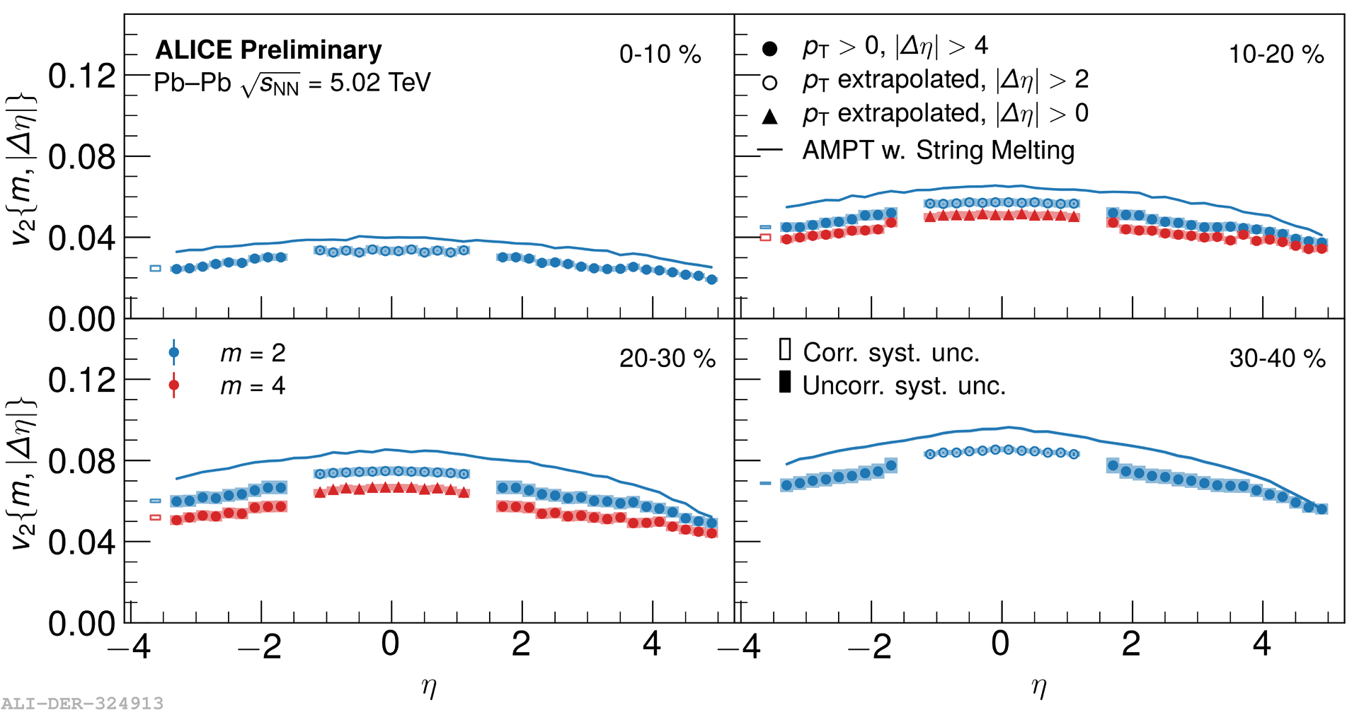
AMPT w. String Melting [Lin, Zi-Wei et al. Phys.Rev. C72 (2005)]
- describes the data qualitatively, but not quantitatively

Figure: $ v_2\{2,|\Delta \eta| > 2\}$ and $v_2\{4,|\Delta \eta| > 0\}$ as a function of $ \eta $.

Introducing 4-particle cumulant and 2-particle cumulant w. a large $ \eta $-gap
Flat shape $ \rightarrow $ Implies small $ \eta $-gap in central heavy ion collisions might not be enough:
- to suppress non-flow
- for factorization

4-particle cumulant and 2-particle cumulant with a large eta-gap

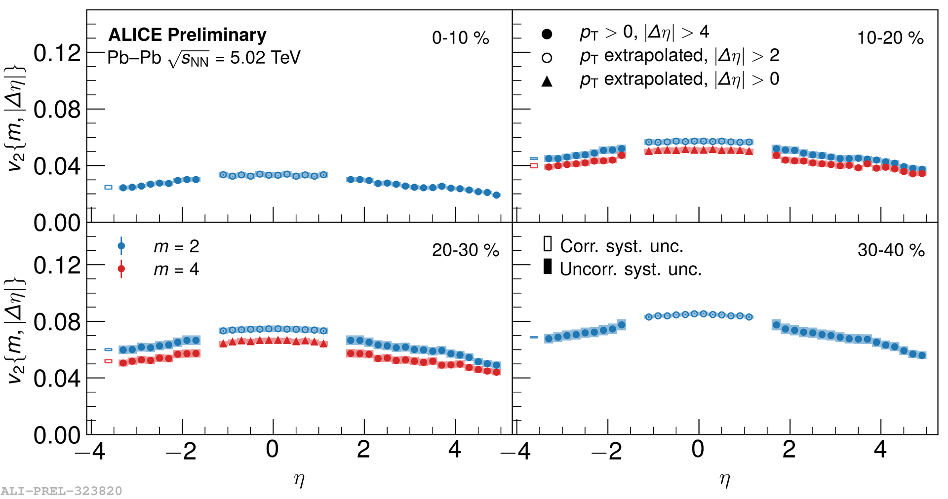
NEW

Figure: $ v_2\{2,|\Delta \eta| > 2\}$ and $v_2\{4,|\Delta \eta| > 0\}$ as a function of $ \eta $.

4-particle cumulant and 2-particle cumulant with a large eta-gap

NEW

Introducing 4-particle cumulant and 2-particle cumulant w. a large $ \eta $-gap
Flat shape $ \rightarrow $ Implies small $ \eta $-gap in central heavy ion collisions might not be enough:
- to suppress non-flow
- for factorization
AMPT w. String Melting [Lin, Zi-Wei et al. Phys.Rev. C72 (2005)]
- describes the data qualitatively, but not quantitatively

summary and overview

$v_n (\eta)$ with Pb-Pb 5.02 TeV in a wide range in pseudorapidity
$ v_n $ measured w. large gap and 4-particle cumulant: more flat shape than $ v_n $ w. a small gap
AMPT has qualitative agreement, but improvements are needed
Future comparisons to 3+1D hydrodynamic calculations:
- can constrain the initial state models
- study longitudinal dynamics of the created hot and dense matter

summary

back-up slides

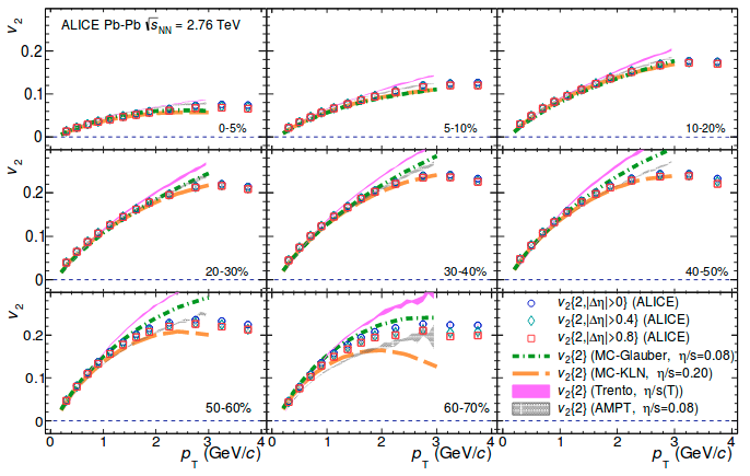
Figure: $ p_T$ differential flow measurements.

[ALICE Collaboration, JHEP 1709 (2017)]

FMD measure all charged particles, i.e. $ p_T > 0 $ GeV/c
TPC measure charged particles with
$ p_T > 0.2 $ GeV/c
- additional cut $p_T < 5$ GeV/c
This will increase flow in TPC, wrt. the FMD
- is corrected with MC

momentum in the fmd and tpc

Figure: Data points: $ v_n \{ 2\},|\Delta \eta|> 0 $ in Pb-Pb 5.02 TeV.
Boxes: Standard Q-cumulant $ v_n \{ 2\} $ from [ALICE Collaboration,
Phys.Lett. B762 (2016)] in Pb-Pb 2.76 TeV.

pseudorapidity dependence on vn in pb-pb 2.76 tev

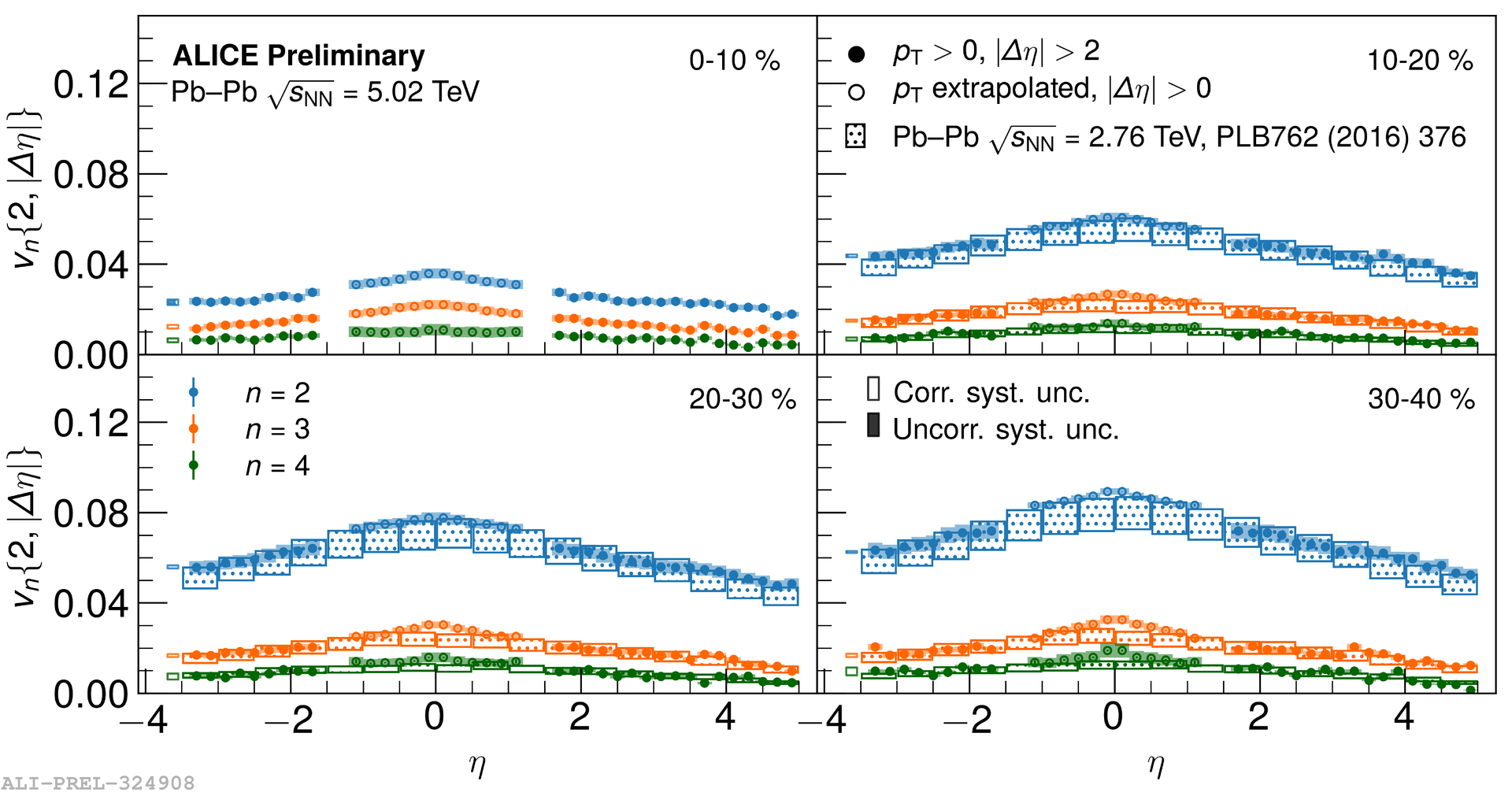
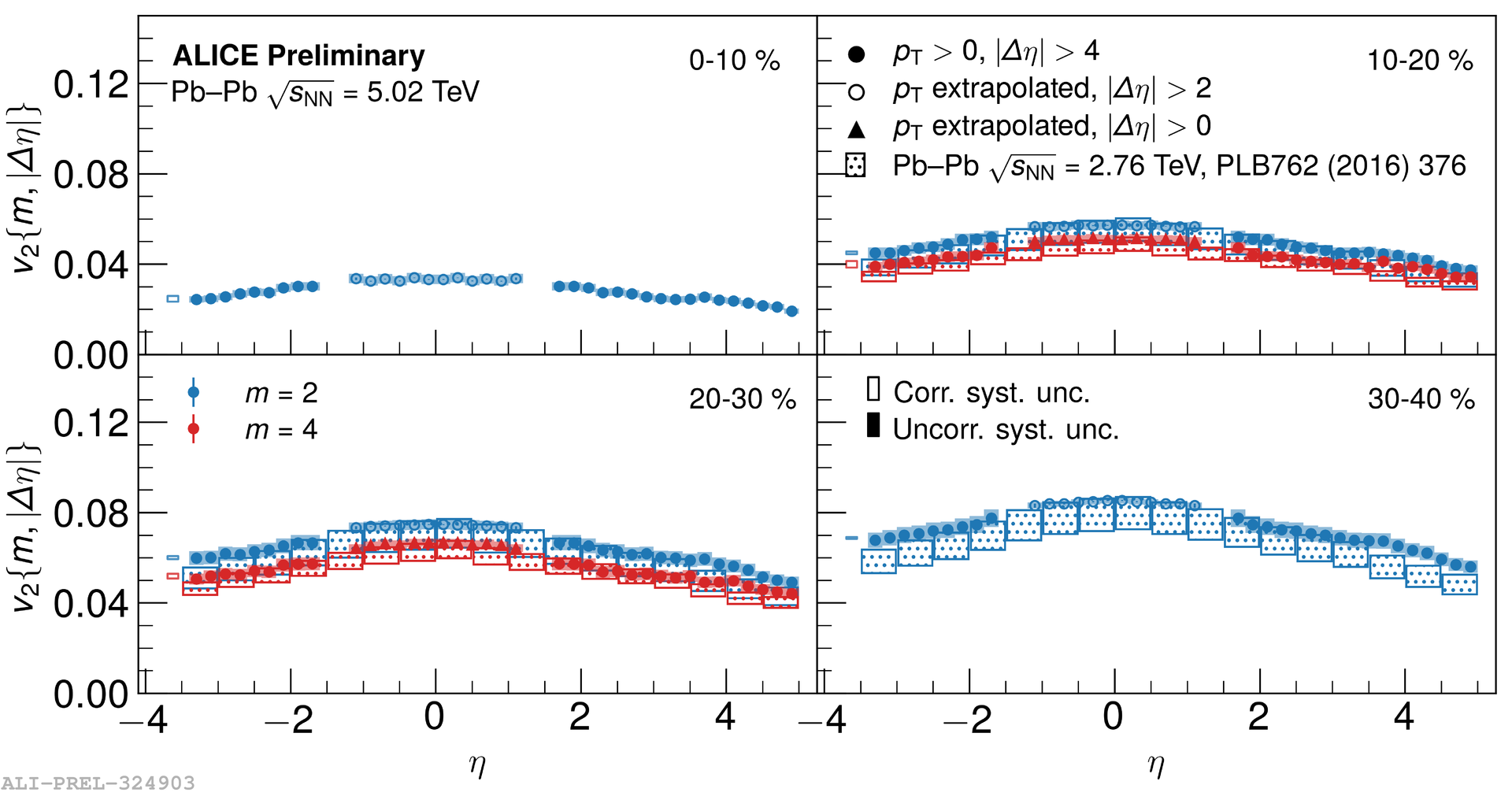
Figure: Data points: $ v_2 \{ 2\},|\Delta \eta|> 2 $ and $ v_2 \{ 4\},|\Delta \eta|> 0 $ in Pb-Pb 5.02 TeV.
Boxes: Standard Q-cumulant $ v_2 \{ 2\} $ and $ v_2 \{ 4\} $ from [ALICE Collaboration, Phys.Lett. B762 (2016)] in Pb-Pb 2.76 TeV.

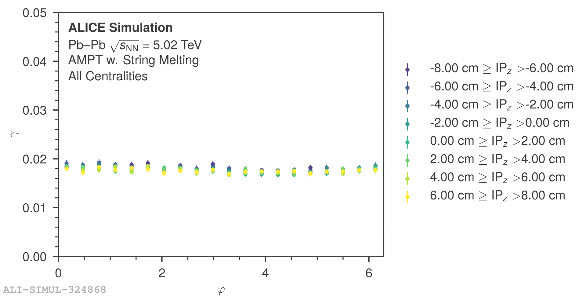
Analysis repeated in $ \eta $
- $ \Delta \eta $ of observed secondary particle to primary particle
- Fourier transform $ f(\eta) $ for each vertex and $ \varphi $ bin
Width of peaks are constant at 0.02

secondaries in the fmd

Figure: Widths of peaks of the distributions.

Figure: Distribution of a secondary particle around its primary mother particle. Plots are shifted by a constant.

secondaries in the fmd - correction to v3 and v4

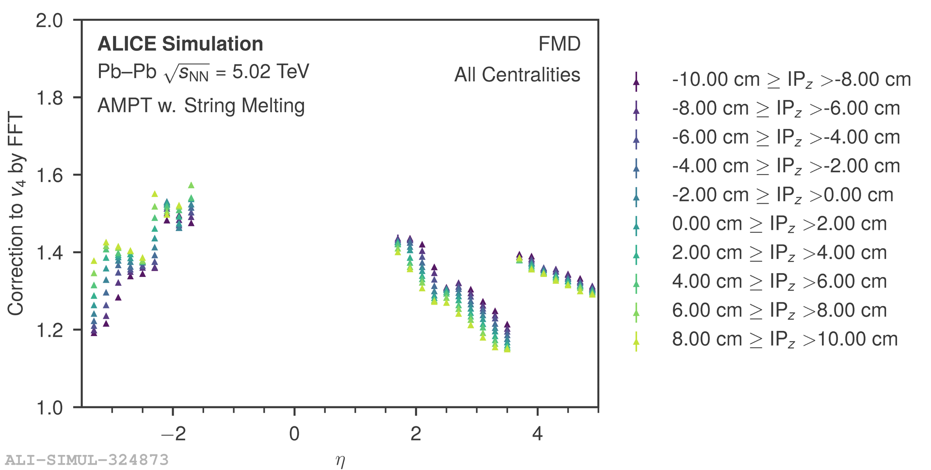
Figure: Correction to $v_3$ for the contamination of secondary particles in the FMD.

Pseudorapidity dependence of anisotropic flow in heavy ion collisions with ALICE

introduction

anisotropic flow

anisotropic flow

flow as a function of pseudorapidity

flow as a function of pseudorapidity

experiment

alice

methods

generic framework

non-flow suppression using eta-gaps

estimating factorising limit

sub-events with pseudorapidity gap

Secondaries in the forward multiplicity detector

distribution of secondary particles from material

smearing by secondary particles

distribution of secondaries around primary particles

results

pb-pb

two particle cumulant with small eta-gap

two particle cumulant with small eta-gap

4-particle cumulant and 2-particle cumulant with a large eta-gap

4-particle cumulant and 2-particle cumulant with a large eta-gap

summary and overview

summary

back-up slides

momentum in the fmd and tpc

pseudorapidity dependence on vn in pb-pb 2.76 tev

secondaries in the fmd

secondaries in the fmd - correction to v3 and v4